Speculative Decoding: From Theory to Implementation

Let's talk about speculative decoding. One of the most elegant optimization techniques in modern LLM inference. If you've ever wondered how to squeeze 2-3x more throughput from your language models without sacrificing output quality, you're in the right place.

By the end of this post, you'll understand the algorithm deeply enough to implement it from scratch. We'll cover the motivation, the math, the implementation details, and the subtle edge cases that make or break a real-world deployment.

The Problem: Autoregressive Decoding is Memory-Bound

When a large language model generates text, it does so autoregressively: one token at a time. Here's what happens at each step:

1. Load model weights from memory (billions of parameters)

2. Compute attention over all previous tokens

3. Generate logits for the next token

4. Sample or argmax to pick the next token

5. Repeat

The problem? Modern GPUs are incredibly powerful at computation but relatively slow at memory access. When you generate a single token, you're moving gigabytes of weights from HBM (high-bandwidth memory) to compute units, performing trillions of operations, and producing... one token.

This is called being memory-bandwidth bound. Your compute units are sitting idle most of the time, waiting for data to arrive. For a 70B parameter model in BF16, you're loading ~140GB of weights per token. If your GPU has 2TB/s memory bandwidth, that's a theoretical minimum of 70ms per token, regardless of how fast your compute is.

So, how can we be more efficient?

Speculative Decoding

The answer is Speculative Decoding and the key idea behind this technique is that verifying K tokens takes roughly the same time as generating 1 token.

Let's make this concrete with an example. Suppose you're using GPT-2-XL and you've generated the sequence:

"The capital of France is"

Standard Approach: One Token at a Time

Normally, to generate the next 4 tokens, you'd do:

Step 1: Forward pass with "The capital of France is" → generate "Paris"
Step 2: Forward pass with "The capital of France is Paris" → generate ","
Step 3: Forward pass with "The capital of France is Paris," → generate "which"
Step 4: Forward pass with "The capital of France is Paris, which" → generate "is"

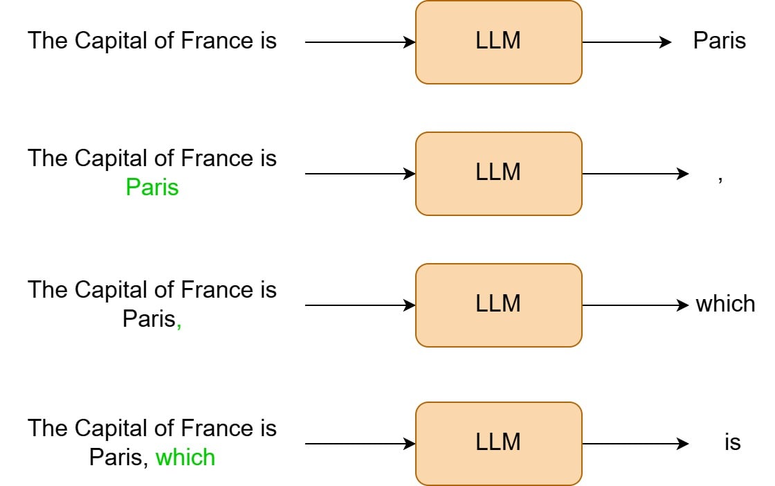
Total: 4 forward passes through GPT-2-XL

Each forward pass loads all 1.5 billion parameters from memory and runs attention over the entire sequence. If each pass takes 100ms, that's 400ms total.

Speculative Approach: Verify Multiple Tokens at Once

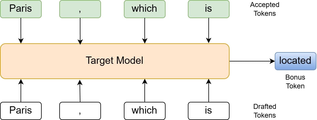
Now imagine you have a small GPT-2 model that can guess these 4 tokens ahead of time. You create the sequence:

"The capital of France is Paris, which is"

And you do one forward pass through GPT-2-XL with this entire sequence. This single pass gives you:

• Logits at position "is" (after "France is") → to verify "Paris"

• Logits at position "Paris" → to verify ","

• Logits at position "," → to verify "which"

• Logits at position "which" → to verify "is"

• Logits at position "is" → bonus token for free!

Total: 1 forward pass through GPT-2-XL

Why Does This Take the Same Time?

When you verify K tokens, you're:

1. Loading the model weights once (same cost)
   Whether you're processing "The capital of France is" (5 tokens) or "The capital of France is Paris, which is" (9 tokens), you still load the same 1.5B parameters from memory. This is the expensive part and it doesn't change.

2. Running attention over a sequence that's K tokens longer (negligible cost for small K)
   Yes, computing attention over 9 tokens instead of 5 tokens is slightly more work. But this is compute-bound work, not memory-bound. Your GPU has thousands of cores sitting idle during the memory load. The extra computation is essentially free as it happens while waiting for memory anyway. For small K (like 3-5 tokens), this adds maybe 5-10ms to a 100ms forward pass. Negligible.

   (And trust me, having compute bound problems is the best kind of problems to have)

3. Getting K logit outputs instead of 1 (free since we're compute-bound on this part)
   A transformer doesn't just output logits at the last position but it outputs logits at every position in the sequence. We usually throw away all but the last one. In speculative decoding, we actually use them to verify our guesses. Computing logits for 9 positions vs 5 positions? That's just a few extra matrix multiplications, which happen in parallel. Essentially free.

Magic Moments: Cheap Guesses + Fast Verification

So, here's the full picture:

• Cost of 4 separate GPT-2-XL forward passes: 400ms

• Cost of 4 GPT-2 guesses: 4 × 8ms = 32ms

• Cost of 1 GPT-2-XL verification pass: 105ms (slightly longer due to 4 extra tokens)

• Total speculative cost: 32ms + 105ms = 137ms

Speedup: 400ms / 137ms ≈ 2.9x

And this assumes all guesses are correct! Even if only 50% of guesses are right, you still come out way ahead.

The key insight: if you can guess tokens cheaply (using a small model), verifying them all at once is nearly free. You've just turned a sequential problem into a partially parallel one.

The Algorithm: Draft, Verify, Accept

Let’s dive deeper into the algorithm for speculative decoding and try to build it from scratch:

Phase 1: Drafting

Use a small, fast "draft model" to generate K tokens autoregressively. This model should be:

• Much smaller than your target model (10-100x fewer parameters)

• Fast enough that generating K tokens is cheaper than one target model forward pass

• Similar enough to the target model that it gets some tokens right

Here's how we implement the drafting phase:

def generate_draft_tokens(self, input_ids: torch.Tensor, num_tokens: int) -> Tuple[List[int], List[float]]:
    """
    Use the draft model to generate candidate tokens.

    Args:
        input_ids: Current token sequence
        num_tokens: Number of tokens to draft

    Returns:
        Tuple of (draft_tokens, draft_probabilities)
    """
    draft_tokens = []
    draft_probs = []

    current_ids = input_ids.clone()

    for _ in range(num_tokens):
        with torch.no_grad():
            outputs = self.draft_model(current_ids)
            logits = outputs.logits[0, -1, :]  # Last position
            probs = torch.softmax(logits, dim=0)

            # Sample next token
            next_token = torch.multinomial(probs, num_samples=1)
            token_id = next_token.item()

            draft_tokens.append(token_id)
            draft_probs.append(probs[token_id].item())

            # Append token for next iteration
            current_ids = torch.cat([current_ids, next_token.unsqueeze(0)], dim=1)

    return draft_tokens, draft_probs

The critical detail: we store both the tokens AND their probabilities under the draft model. We'll need draft_probs for the acceptance step.

Phase 2: Verification

This is where the magic happens. Take all K draft tokens and run them through the target model in one forward pass.

# Create sequence with all draft tokens
draft_sequence = torch.cat([
    input_ids,
    torch.tensor([draft_tokens], device=self.device)
], dim=1)

# Single forward pass through target model
with torch.no_grad():
    outputs = self.target_model(draft_sequence)
    all_logits = outputs.logits[0]  # Shape: [seq_len, vocab_size]

Notice what we're doing: we're feeding the entire sequence (original input + all K draft tokens) into the target model at once. The output gives us logits at every position, which means we get probability distributions for verifying each draft token.

This is the key efficiency gain. Instead of K separate forward passes (one per token), we do one forward pass that's slightly longer.

Phase 3: Acceptance with Rejection Sampling

Now comes the subtle part: we need to accept or reject each draft token in a way that preserves the exact probability distribution of the target model.

def verify_draft_tokens(self, input_ids: torch.Tensor, 
                       draft_tokens: List[int], 
                       draft_probs: List[float]) -> List[int]:
    """
    Verify draft tokens using the target model in a single forward pass.

    This is where the magic happens! We process all draft tokens at once
    and get probability distributions at each position.
    """
    # Create sequence with all draft tokens
    draft_sequence = torch.cat([
        input_ids,
        torch.tensor([draft_tokens], device=self.device)
    ], dim=1)

    # Single forward pass through target model
    with torch.no_grad():
        outputs = self.target_model(draft_sequence)
        all_logits = outputs.logits[0]  # Shape: [seq_len, vocab_size]

    # Verify each draft token
    accepted_tokens = []
    seq_len = input_ids.size(1)

    for i in range(len(draft_tokens)):
        # Get target model's probability distribution at this position
        position = seq_len - 1 + i
        target_probs = torch.softmax(all_logits[position], dim=0)
        target_prob = target_probs[draft_tokens[i]].item()
        draft_prob = draft_probs[i]

        # Acceptance criterion: p_target(token) / p_draft(token)
        acceptance_ratio = min(1.0, target_prob / draft_prob)

        if torch.rand(1).item() < acceptance_ratio:
            # Accept the draft token
            accepted_tokens.append(draft_tokens[i])
        else:
            # Reject and sample from adjusted distribution
            # Adjusted distribution: max(0, p_target - p_draft)
            adjusted_probs = torch.clamp(
                target_probs - torch.softmax(all_logits[position], dim=0), 
                min=0.0
            )

            if adjusted_probs.sum() > 0:
                adjusted_probs = adjusted_probs / adjusted_probs.sum()
                new_token = torch.multinomial(adjusted_probs, num_samples=1).item()
            else:
                # Fallback: sample from target distribution
                new_token = torch.multinomial(target_probs, num_samples=1).item()

            accepted_tokens.append(new_token)
            # Stop verifying remaining tokens
            break

    # Bonus token: if all drafts accepted, get one more from target model
    if len(accepted_tokens) == len(draft_tokens):
        position = seq_len - 1 + len(draft_tokens)
        bonus_probs = torch.softmax(all_logits[position], dim=0)
        bonus_token = torch.multinomial(bonus_probs, num_samples=1).item()
        accepted_tokens.append(bonus_token)

    return accepted_tokens

Let's break down what's happening in the acceptance loop:

The Math: Understanding Rejection Sampling

At each position i, we have:

• p_target: the target model's probability for the draft token

• p_draft: the draft model's probability for that token (which we stored earlier)

The acceptance probability is:

acceptance_ratio = min(1.0, p_target / p_draft)

Why This Formula?

Case 1: p_target ≥ p_draft
The target model thinks this token is more likely than the draft model did. Accept it with probability 1.0. The draft model was being conservative, which is fine.

Case 2: p_target < p_draft
The draft model was overly confident. We accept with probability p_target / p_draft, which downweights based on how overconfident the draft was.

For example:

• If p_draft = 0.8 and p_target = 0.4, we accept with probability 0.4/0.8 = 0.5

• If p_draft = 0.9 and p_target = 0.1, we accept with probability 0.1/0.9 ≈ 0.11

The Adjusted Distribution

When we reject a token, we can't just sample from the target model's distribution directly as that would create bias. Instead, we sample from an adjusted distribution:

p'(t) = max(0, p_target(t) - p_draft(t)) / Z

Where Z is a normalization constant. This adjustment removes the "contribution" of the draft model, leaving only what the target model adds.

The intuition: the draft model already "used up" some probability mass on the token it sampled. We need to sample from what's left over.

adjusted_probs = torch.clamp(
    target_probs - torch.softmax(all_logits[position], dim=0), 
    min=0.0
)

if adjusted_probs.sum() > 0:
    adjusted_probs = adjusted_probs / adjusted_probs.sum()
    new_token = torch.multinomial(adjusted_probs, num_samples=1).item()

This rejection sampling procedure is mathematically proven to produce the exact same distribution as standard autoregressive decoding. So, you're not approximating but getting bit-for-bit identical results (in expectation).

The Bonus Token

There's one more clever optimization:

# Bonus token: if all drafts accepted, get one more from target model
if len(accepted_tokens) == len(draft_tokens):
    position = seq_len - 1 + len(draft_tokens)
    bonus_probs = torch.softmax(all_logits[position], dim=0)
    bonus_token = torch.multinomial(bonus_probs, num_samples=1).item()
    accepted_tokens.append(bonus_token)

If all K draft tokens were accepted, we got K+1 positions worth of logits from the target model (the original K positions plus one more). That extra position is essentially free since we already paid the cost of the forward pass. So, we sample one more token from it.

This means a perfect draft gets you K+1 tokens for the price of one target model pass!

Putting It All Together

Here's the complete generation loop:

def generate(self, prompt: str, max_new_tokens: int = 50, 
             num_draft_tokens: int = 4, verbose: bool = True) -> str:
    """
    Generate text using speculative decoding.
    """
    input_ids = self.tokenizer.encode(prompt, return_tensors='pt').to(self.device)
    generated_tokens = 0
    iterations = 0
    total_accepted = 0

    while generated_tokens < max_new_tokens:
        iterations += 1

        # Step 1: Draft tokens
        draft_tokens, draft_probs = self.generate_draft_tokens(input_ids, num_draft_tokens)

        # Step 2: Verify drafts
        accepted_tokens = self.verify_draft_tokens(input_ids, draft_tokens, draft_probs)

        # Update statistics
        num_accepted = len(accepted_tokens)
        total_accepted += num_accepted
        generated_tokens += num_accepted

        if verbose:
            draft_text = self.tokenizer.decode(draft_tokens)
            accepted_text = self.tokenizer.decode(accepted_tokens)
            print(f"Iteration {iterations}:")
            print(f"  Drafted: {draft_text!r}")
            print(f"  Accepted: {accepted_text!r} ({num_accepted}/{len(draft_tokens)} tokens)")

        # Add accepted tokens to sequence
        input_ids = torch.cat([
            input_ids,
            torch.tensor([accepted_tokens], device=self.device)
        ], dim=1)

        if generated_tokens >= max_new_tokens:
            break

    result = self.tokenizer.decode(input_ids[0], skip_special_tokens=True)
    return result

Each iteration:

1. Drafts K tokens using the small model

2. Verifies all K tokens in one pass through the large model

3. Accepts between 1 and K+1 tokens

4. Repeats until we've generated enough tokens

Setting Up the Models

To use speculative decoding, you need two models from the same family:

class SpeculativeDecoder:
    def __init__(self, draft_model_name: str, target_model_name: str):
        """
        Initialize the speculative decoder with two models.

        Args:
            draft_model_name: Name of the small, fast model (e.g., "gpt2")
            target_model_name: Name of the large, accurate model (e.g., "gpt2-xl")
        """
        print(f"Loading draft model: {draft_model_name}")
        self.draft_model = AutoModelForCausalLM.from_pretrained(draft_model_name)
        self.draft_model.eval()

        print(f"Loading target model: {target_model_name}")
        self.target_model = AutoModelForCausalLM.from_pretrained(target_model_name)
        self.target_model.eval()

        self.tokenizer = AutoTokenizer.from_pretrained(draft_model_name)
        self.tokenizer.pad_token = self.tokenizer.eos_token

        # Move to GPU if available
        self.device = "cuda" if torch.cuda.is_available() else "cpu"
        self.draft_model.to(self.device)
        self.target_model.to(self.device)

In this example, we use GPT-2 (124M parameters) as the draft model and GPT-2-XL (1.5B parameters) as the target. The draft model is roughly 12x smaller, which translates to roughly 12x faster inference.

Important: both models must use the same tokenizer and vocabulary. Otherwise, you'd need token mapping logic, which adds complexity.

Performance Analysis

Let's analyze the theoretical speedup. Define:

• T_target: time for one target model forward pass

• T_draft: time for one draft model forward pass

• α: average acceptance rate aka block efficiency (probability a draft token is accepted)

• K: number of draft tokens per iteration

Time per iteration:

T_iteration = K × T_draft + T_target

Expected tokens per iteration:

This is trickier. If each token has independent acceptance probability α, the expected number of accepted tokens is:

E[tokens] = 1 + α + α² + α³ + ... + α^(K-1) + α^K
          = (1 - α^(K+1)) / (1 - α)

For large K and reasonable α, this approximately equals:

E[tokens] ≈ 1 / (1 - α)

Effective time per token:

T_effective = (K × T_draft + T_target) / E[tokens]

Example Calculation

Let's use realistic numbers:

• T_target = 100ms (GPT-2-XL on GPU)

• T_draft = 8ms (GPT-2 on same GPU, ~12x faster)

• K = 4 (draft 4 tokens)

• α = 0.6 (60% acceptance rate)

T_iteration = 4 × 8ms + 100ms = 132ms
E[tokens] = (1 - 0.6^5) / (1 - 0.6) ≈ 2.2 tokens
T_effective = 132ms / 2.2 ≈ 60ms per token

Speedup: 100ms / 60ms ≈ 1.67x

And this is without KV caching! With proper KV cache management, the speedup can reach 2-3x.

Optimal K Value

The choice of K (number of draft tokens) is a tradeoff:

• Too small: You don't utilize the verification pass fully

• Too large: You waste time drafting tokens that will be rejected

The optimal K depends on:

1. The speed ratio between models (T_target / T_draft)

2. The acceptance rate α

3. Memory constraints

In practice, K=3 to K=5 works well for most scenarios.

Acceptance Rate in Practice

What determines the acceptance rate? Several factors:

Model Similarity: Draft and target models from the same family (GPT-2 → GPT-2-XL) have higher acceptance rates than mismatched models.

Task Difficulty:

• Predictable text (news articles, documentation): α ≈ 0.7

• Creative writing: α ≈ 0.4-0.5

• Code generation: α ≈ 0.5-0.6

Context Length: Acceptance rate often improves with longer context as more information makes tokens more predictable.

Temperature: Lower temperature (greedier) typically gives higher acceptance rates because both models converge toward obvious choices.

Here's what you'll see when running the code:

Iteration 1:
  Drafted: ' a topic that'
  Accepted: ' a topic' (2/4 tokens)

Iteration 2:
  Drafted: ' that has been'
  Accepted: ' that has been' (4/4 tokens)

Iteration 3:
  Drafted: ' discussed extensively'
  Accepted: ' discussed' (1/4 tokens)

The variation is normal! Some iterations accept everything, some only accept one token.

Implementation Considerations

Memory Requirements

You need to keep both models in memory simultaneously. For GPT-2/GPT-2-XL:

• GPT-2: ~500MB

• GPT-2-XL: ~6GB

• Total: ~6.5GB

For larger models like LLaMA-7B (draft) and LLaMA-70B (target), you're looking at ~14GB + ~140GB ≈ 150GB+. This often requires multiple GPUs.

KV Cache Support

The implementation above doesn't use KV caching, which means we're recomputing attention for all previous tokens at every step. Adding KV cache support significantly improves performance:

1. Draft model cache: Maintain a separate KV cache for drafting

2. Target model cache: Cache verified prefixes only

3. Cache invalidation: When rejecting tokens, truncate the cache to the rejection point

With KV caching, you can achieve 2-3x speedups instead of ~1.5-2x.

Batch Size Considerations

Speculative decoding with batched inference is tricky. Different sequences in the batch may accept different numbers of tokens, creating ragged tensors.

Solutions:

• Independent processing: Process each sequence separately (simpler but less efficient)

• Padding: Pad to max accepted length (wastes computation on padding)

• Dynamic batching: Use frameworks that handle variable-length sequences efficiently

Most production systems use independent processing for simplicity.

Greedy vs. Sampling

The implementation above uses sampling (torch.multinomial). For greedy decoding, you can simplify:

# Greedy acceptance: just check if draft token matches argmax
target_token = torch.argmax(target_probs)
if draft_tokens[i] == target_token:
    accepted_tokens.append(draft_tokens[i])
else:
    accepted_tokens.append(target_token)
    break

Greedy decoding typically has higher acceptance rates because both models converge to the same obvious choice.

When Speculative Decoding Excels

Not all scenarios benefit equally. Here's where it shines:

✅ Large model + small draft model (>10x size difference)
The bigger the speed gap, the more you gain.

✅ Medium to high acceptance rates (>40%)
If your draft model is terrible, the overhead dominates.

✅ Single-user or small-batch inference
Easier to manage than large batches.

✅ Moderate context lengths (<8K tokens)
Very long contexts make verification more expensive.

✅ Predictable tasks
Question answering, summarization, translation work better than creative writing.

When It Struggles

❌ Small target models
If your target model is already fast (<20ms/token), the absolute gains are minimal.

❌ Low acceptance rates (<30%)
Draft overhead exceeds gains.

❌ Very long contexts (>32K tokens)
Verification pass becomes expensive.

❌ Highly creative tasks
Low perplexity means less predictability, lower acceptance rates.

❌ Memory-constrained environments
Keeping two models in memory is a luxury.

Wrapping Up

Speculative decoding is a beautiful example of turning a sequential problem into a partially parallel one. The key insights:

1. Memory bandwidth, not compute, is the bottleneck in LLM inference

2. Verification is nearly free because it's one forward pass regardless of K

3. Rejection sampling preserves distributional correctness so you get exact results

4. Most tokens are predictable making draft models surprisingly effective

The implementation requires careful handling of:

• Rejection sampling math to maintain correctness

• Probability tracking for both draft and target models

• Early stopping when rejecting tokens

• Bonus token extraction for efficiency

The result? 1.5-3x speedup on real workloads with zero quality degradation. Not bad for a technique that's conceptually just "guess and check."

If you're deploying LLMs at scale, speculative decoding should be in your optimization toolkit. The math is subtle, but the payoff is real.

---

Full working code available at: github.com/jaygala223/scratch

Try it yourself:

python3 speculative_decoding.py

And watch as your LLM generates text faster without sacrificing a single bit of quality.